Post by Aadith Vittala.

This paper serves as a review of similarity-based online unsupervised learning algorithms. These types of algorithms are important because they are biologically-plausible, produce non-trivial results, and sometimes work as well as other non-biological algorithms. In this paper, biologically-plausible algorithms have three main features: they are local (each neuron uses only pre or post synaptic information), they are online (data vectors are presented one at a time and learning occurs after each data vector is passed in), and they are unsupervised (there is no teaching signal to tell the neurons information about error). The simplest example of one of these algorithms is the Oja online PCA algorithm. Here, the system receives each timestep and calculates , which represents the value of the top principal component. The weights are modified each timestep according to

This algorithm is both biologically-plausible and potentially useful. This paper aims to find more algorithms like the Oja online PCA algorithm.

As a starting point, they aimed to develop a biologically-plausible algorithm that would output multiple principal components from a given data set. To do this, they chose to use a similarity-matching objective function, where the goal is to minimize the following expression

This expression essentially tries to match the pairwise similarities between input vectors to the pairwise similarities between output vectors. In previous work, they have shown that the solution to this problem (with having fewer dimensions than ) is PCA. To solve this in a biologically-plausible fashion, they use a variable substitution trick (inspired by the Hubbard-Stratonovich transformation from physics) to convert this problem to a minimax problem over new variables and

This expression leads to an online algorithm where you solve for during each time step using

and then update and with

though after discussion, we think it would be better to call the second weights update “Hebbian for inhibitory synapses”. This online algorithm has not yet been proven to converge, but it gives relatively good results when tested. In addition, it provides a simple interpretation of as the presynaptic weights mapping all inputs to all neurons, as the postsynaptic output from all neurons, and as inhibitory lateral projections between neurons.

The paper goes on to generalize this algorithm to accept whitening constraints (via Lagrange multipliers), to work for non-negative outputs, and to work for clustering and manifold tiling. The details for all of these processes are covered in cited papers, but not in this specific paper. Overall, the similarity-matching objective seems to give well-performing biologically-plausible algorithms for a wide range of problems. However, there are a few important caveats: none of these online algorithms have been proved to converge for the correct solution, inputs were not allowed to correlate, and there is no theoretical basis for stacking (since multiple layers would be equivalent to a single layer). In addition, during discussion we noted that similarity matching seems to essentially promote networks that just rotate their input into their output (as similarity measures the geometric dot product between vectors), so it is not obvious how this technique can conduct the more non-linear transformations necessary for complex computation. Nonetheless, this paper and similarity-matching in general provides important insight into how networks can perform computations while still remaining within the confines of biological plausibility. 

I make a distinction between latent variables and parameters. Latent variables change over time; parameters don’t.

(This is really a quantitative matter, not a qualitative one, as a “parameter” might change slowly (often called adaptation) and thus be promoted to a “variable.”)

This distinction carries over to computation: inferring a variable is just called “inference,” but inferring a parameter is typically called “learning.” Mathematically, these are really the same process, just about different quantities and on different timescales.

Analogously, model bias and inductive bias are both biases, but about variables versus parameters. Model bias is an inference bias in the mapping from input to output. Inductive bias is a learning bias, a bias in what is learned from data (i.e. in the mapping from a data set to parameters). This inductive bias in turn creates its own model bias.

An inductive bias is caused by both the model class (such as a neural network architecture) and the optimization procedure.

The following table compares the relevant concepts.

Table: Comparison of latent variables and parameters, and computations relevant to them. Here x is a vector of latent variables, Q is a parameter vector, d is observable input data, {d} is a data set, and M is a model class.

A Task-Optimized Neural Network Replicated Human Auditory Behavior Predicts Brain Responses, and Reveals a Cortical Processing Hierarchy

By  Alexander Kell, Dan Yamins, Erica Shook, Sam V. Norman-Haignere, Josh H. McDermott

Summary by Josue Ortega-Caro

In this work, the authors study the capabilities of a deep neural network to predict both neural responses of human auditory cortex and the behavior of human participants. In addition, the authors point to their results as evidence of hierarchical processing in the auditory cortex. Their results are part of a growing body of work that uses deep neural networks as models of human cortex (see [1] for references), especially the visual cortex.

The assumption behind this literature states that everyday perceptual tasks may impose strong constraints on the brain. These constraints may yield general principles of how tasks can be solved within a distributed network architecture. Therefore, deep neural networks trained directly on these perceptual tasks are likely to implement the same solutions as the cortex, and thereby exhibit brain-like representations and transformations.

Through comparisons to humans in several different noise conditions, the authors show the strong similarities between their models and humans in speech and music recognition tasks. These results suggest that deep neural networks also provide a good model for auditory cortex.

The authors used two tasks: speech and music recognition tasks. Every signal was preprocessed by transforming into a cochleogram prior to passing through the network. On the first task, subjects were given a two second clip of speech, and were asked to recognize one of 587 possible words in the middle of a sentence. On the second task, subjects listened to a two second clip of a song, and were asked to identify one of 41 possible genres to which it belongs. In addition, every two second clip was perturbed by different types and levels of background noise, as a way to compare the models’ and humans’ abilities to perform auditory recognition under difficult conditions.

First, the authors performed an architecture search over 180 architectures to find neural networks that perform well on speech and music recognition independently. Next they searched for ways to combine the architectures into a single network that performed both tasks. The authors argue that both speech and music recognition should share low-level auditory features similar to visual recognition tasks. (It was not clear why they wanted to combine networks trained on each task, except perhaps as a way of decreasing the number of parameters needed for both tasks together.) The final network has three parts: a shared-core (up to Conv3) for both tasks, followed by a word-classifier and a genre-classifier branches, selected by the performance on both the speech and music recognition tasks.

The authors compare the behavior (performance) of the model and humans under different noise conditions. Figure 2 shows that under five types of noise at six intensity levels, the human and model behavior have values of 0.25 and 0.92 for music and speech recognition, respectively. One concern during the discussion was the inter-human variance in the task (via between humans), because if humans cannot do this task, consistently, then the small between the model and humans (For music recognition) is a better result. An important caveat stated by the authors is that the genre recognition task has very fine distinction between genres, e.g. “New Age” versus “Ambient”. Therefore, human subjects were asked to perform top-5 categorization.

Moreover, they tested the ability of the model trained on speech and music recognition to predict fMRI recordings of 8 participants to 165 natural sounds. Some of these sounds were speech and music related but most (113 out of 165) were not. They did independent linear readouts from the activations of different layers of their network in order to find which layers better predict each voxel response to the 165 natural sounds. Figure 3 shows that median variance explained by their model is higher than a spatiotemporal model (baseline model) and a random network baseline. This shows that training the model did help its predictive power.

The most interesting results comes when they examine the fine-grain predictions of different model layers for different voxels in the auditory hierarchy. In Figure 4, their hierarchical map shows higher correlation between early layers of auditory cortex and the predicted voxels from the shared-core layers. At the same time, higher cortical areas have higher correlation with their respective task specific branch. In addition, they show that even though the shared layers can predict the higher cortical areas, the specific branches predict significantly better those areas compare to the shared-core and vice versa. Furthermore, music and speech specific voxels are better predicted by their respective branches of the model. Even though this result is very clear, we were not completely sure if the correlation differences are significant between speech and music branches.

Moreover, the authors explore the ability of their model to explicitly represent acoustic features of the stimulus (via linear decodability). They argue that this is a way to understand the representation learned by the model. They show the variance explained of the spectral filters is higher in early layers, and that variance explained of the spectral modulation peaks at intermediate layers. In contrast, the untrained network has a similar profile but not the same increase or decrease in decodability as the trained network. One experiment they might have done is linearly decode of the spectral filters on the fMRI data and see if the voxels that have higher decodability also have high correlation with the early layers of the network.

Lastly, the authors show in Figure 7 that networks at intermediate points during training explain variance that is correlated to its performance in the speech and music tasks. I think this is the clearest result of their philosophical position: There is a linear relationship between the network’s performance on an everyday task, and the presence of brain-like representational transformations.

In conclusion, the authors show a correlation between humans and deep neural networks in neural, behavioral and representational axis during speech and music recognition tasks. As stated before, this framework of task-optimized neural networks is becoming widespread throughout the neuroscience community, going from visual cortex [1], motor cortex [2], etc., and now to auditory cortex. It is important to note, as also noted by the authors, that the behavioral, neural and representational comparison done by the authors are only sufficient to suggest correlations between humans and deep neural networks. We still need more causal ways to compare both systems in order to see if the similarities are superficial (merely because of the highly-optimized nature of both humans and models on speech and music tasks) or if they reveal a deeper relationship between deep neural models and humans. In addition, we wondered if including other neural motifs such as recurrence, feedback modulation and cell-specific functions would help improve the results presented in this paper.

[1] Yamins, D. L., Hong, H., Cadieu, C. F., Solomon, E. A., Seibert, D., & DiCarlo, J. J. (2014). Performance-optimized hierarchical models predict neural responses in higher visual cortex. Proceedings of the National Academy of Sciences, 111(23), 8619-8624.

[2] Michaels, J. A., Dann, B., Intveld, R. W., & Scherberger, H. (2018). Neural dynamics of variable grasp movement preparation in the macaque fronto-parietal network. Journal of Neuroscience, 2557-17.

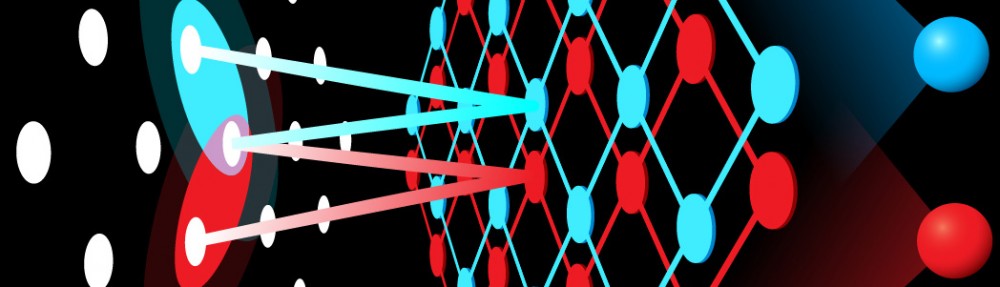
The Sparse Manifold Transform (SMT)

by Yubei Chen, Dylan Paiton, and Bruno Olshausen

https://arxiv.org/abs/1806.08887

Theories of neural computation have included several different ideas: efficient coding, sparse coding, nonlinear transformations, extracting invariances and equivariances, hierarchical probabilistic inference using priors over natural sensory inputs. This paper combined a few of these in a theoretically satisfying way. It is not a machine-learning paper with benchmarks, but is rather a conceptual framework for thinking about neural coding and geometry. It can be applied hierarchically to generate a deep learning method, and the authors are interested in applying this to more complex problems and data sets, but haven’t yet.

The three main ideas synthesized in this paper are: sparse coding, manifold flattening, and continuous representations.

Sparse coding represents an input using an overcomplete basis set (a “dictionary”), by encouraging sparseness (rarity of nonzero coefficients ): . This can be implemented using a biologically plausible neural network that creates a nonnegative sparse code for input with inhibitory lateral connections [Rozell et al 2008].

A manifold is a smooth curved space that is locally isomorphic to a Euclidean space. Natural images are often thought of occupying low-dimensional manifolds embedded within the much larger space of all possible images. That is, any single natural image with pixels is a point that lives in a manifold . Since the intrinsic dimensionality of the manifold is much smaller than the embedding space, we should be able to compress the image by constructing coordinates within the manifold. These intrinsic coordinates could then provide a locally flat space for the data. They may also provide greater interpretability. With some possibly substantial geometric or topological distortions (including rips), the whole manifold could be flattened too.

People have published several ways to flatten manifolds. One prominent one is Locally Linear Embedding [Roweis and Saul 2000], which expresses points on the manifold as linear combinations of nearby data points. A coarser and more compressed variant is Locally Linear Landmarks (LLL) [Vladymyrov M, Carreira-Perpinán 2013] which just uses a smaller set of points as “landmarks” rather than using all data. In both variants, each landmark in the original space is mapped to a landmark in a lower-dimensional space, so that points in the original curved manifold, , are mapped to points in the flat space, , using the same coordinates .

The SMT authors observe that sparse coding and manifold flattening are connected. Since you only use a few landmarks to reconstruct the original signal, the coefficients are sparse: the LLL is a sparse code for the manifold.

Continuous representations: In general, sparse coding does not impose any particular organization on the dictionary elements. One can pre-specify some locality structure to the dictionary, as in Topographic ICA [Hyvärinen et al 2001] which favors dictionary elements that have high similarity to other dictionary elements when and are close. In SMT, the authors propose to find dictionaries in the target space for which smooth trajectories are flat. That is, any representation at time should be halfway between the representations at the previous and next frames: . If the target trajectories are curved, this will not be true. The authors achieve this by minimizing the average second derivative of the data trajectories in the flattened space, . They have an analytic solution that works in some cases, but they use stochastic gradient descent to accommodate more flexible constraints.

The authors relate this idea to Slow Feature Analysis (SFA) [Wiskott and Sejnowski 2002], another unsupervised learning concept that I really like. In SFA, one finds nonlinear transformations that change slowly, according to . The idea is that these directions are features that are invariant to fast changes in the appearance of objects (lighting, pose) and encode instead the consistent properties of those objects. In SMT, this is achieved by minimizing the second derivative of instead of the first.

There’s actually an interesting distinction to be drawn here: their manifold flattening should not throw away information, as do many models for extracting invariances, including SFA. Instead the coordinates on the manifold actually try to represent all relevant directions, and the flat representation ensures that changes in the appearance are equally matched by changes in the representation . This concept is called equivariance. The goal is reformatting for easier access to properties of interest.

Applications

Finally, the authors note that they can apply this method hierarchically, too, to progressively flatten the manifold more and more. Each step expands the representation nonlinearly to obtain a sparse code , and then compresses it to a flatter representation .

They demonstrate their approach on one toy problem for illustration, and then apply it to time sequences of image patches. As in many other methods, they recover Gabor-like features once again, but they discover some locality to their Gabors and smoothness in the sparse coefficients and target representation. When applied iteratively, the Gabors seem to get a bit longer and may find some striped textures, but nothing impressive yet. Again I think the conceptual framework is the real value here. The authors plan on deploying their method on larger scales, and it will be interesting to see what emerges.

Discussion

Besides the foundational concepts (sparse coding, LLL, SFA), the authors only briefly mention other related works. It would be helpful to see this section significantly expanded, both in terms of how the conceptual framework relates to other approaches, and how performance compares.

One fundamental and interesting concept that the authors could elaborate substantially more is how they think of the data manifold. They state that “natural images are not well described as a single point on a continuous manifold of fixed dimensionality,” but that is how I described the manifold above: an image was just a point . Instead they favor viewing images as a function over a manifold. A single location on the manifold is like a 1-sparse function over the manifold (with a fixed amplitude). They prefer instead to allow an -sparse function, i.e. points on the same manifold. I emailed the authors asking for clarification about this, and they graciously answered quickly. Bruno said “an image patch extracted from a natural scene could easily contain two or more edges moving through it in different directions… which you can think of that as two points moving in different trajectories along the same manifold. We would call that a 2-sparse function on the manifold. It is better described this way rather than collapsing the entire image patch into a single point on a bigger manifold, because when you do that the structure of the manifold is going to get very complicated.” This is an interesting perspective, even though it does not come through well in the current version. One crucial thing to highlight from this quote is that the -sparse functions lie on a smaller manifold than the -dimensional image space. What is this smaller manifold? Can it be embedded in the same pixel space? And how do the points on the manifold interact in cases like occlusion or yoked parts?

Yubei suggested this view could have a major benefit to hierarchical inference: “Just like we reuse the pixels for different objects, we can reuse the dictionary elements too. Sparsity models the discreteness of the signal, and manifolds model the continuity of the signal, so we propose that a natural way to combine them is to imagine a sparse function defined on a low dimensional manifold.”

The geometry of the sensory space is quite interesting and important and merits deeper thinking. It would also be interesting to consider how the manifold structure of sensory inputs affects the manifold structure of beliefs (e.g. posterior probabilities) about those inputs. This seems like a job for Information Geometry [Amari and Nagaoka 2007].

References:

Amari SI, Nagaoka H. Methods of information geometry. American Mathematical Soc.; 2007.

Hyvärinen A, Hoyer PO, Inki M. Topographic independent component analysis. Neural computation. 2001 Jul 1;13(7):1527-58.

Roweis ST, Saul LK. Nonlinear dimensionality reduction by locally linear embedding. science. 2000 Dec 22;290(5500):2323-6.

Rozell CJ, Johnson DH, Baraniuk RG, Olshausen BA. Sparse coding via thresholding and local competition in neural circuits. Neural computation. 2008 Oct;20(10):2526-63.

Vladymyrov M, Carreira-Perpinán MA. Locally linear landmarks for large-scale manifold learning. InJoint European Conference on Machine Learning and Knowledge Discovery in Databases 2013 Sep 23 (pp. 256-271). Springer, Berlin, Heidelberg.

Wiskott L, Sejnowski TJ. Slow feature analysis: Unsupervised learning of invariances. Neural computation. 2002 Apr 1;14(4):715-70.

Summary by Alan Akil

In a recent preprint, Mastrogiuseppe and Ostojic discuss an important extension of classical results on neural networks: Theoretical results dating from the late 80s [e.g. Sompolinsky, Cristani and Sommers 1988] show how high-dimensional, random (chaotic) activity arises robustly in networks of rate units whose activity evolves according to

for nonlinear activation functions . However, this classical work assumes that connectivity in the network is unstructured. Mastrogiuseppe  and Ostojic discuss the case when the connectivity matrix has structure that is defined by a low-rank matrix. In particular, they assume that the connectivity is given by a sum of a low-rank and a random matrix, as

where is the disorder strength, is a Gaussian all-to-all random matrix and every element is drawn from a centered normal distribution with variance , and  where and are -dimensional vectors.

Interestingly, the model remains highly tractable: The activity can either be predominantly confined to a few dimensions determined by the (constant) input, and the vectors that define the low-rank component of the connectivity, or it can exhibit high-dimensional chaos, when the unstructured component dominates. The tractability of the model allowed the authors to to design networks that perform specific computations. Moreover, increasing the rank of the structured part of the connectivity leads to networks that can support an ever wider dynamical repertoire, accompanied by an expanding computational capacity.  This allows for the implementation of complex tasks such as context-dependent decision making.

The authors start by studying a recurrent network with a rank-one structured connectivity component and no external input. In this case the network supports four states of spontaneous activity that depend mainly on disorder strength and structure strength.  For instance, strong structure and low disorder lead to heterogeneous firing rates that are approximately constant in time. The most interesting case occurs when the strengths are comparable, leading to a structured chaotic state characterized by approximately one-dimensional dynamics accompanied by high dimensional temporal fluctuations. This state, is characterized by the emergence of very slow timescales, which may be of separate interest [40]. Importantly, the transitions between these four states can be obtained analytically.

Next, the authors examine what happens when a constant, spatially heterogeneous input drives the neurons in the network [e.g. Rajan, Abbott, Sompolinsky 2010]. In this case, the relation between the left and right structure vectors and the input gave rise to different dynamics in the network. The two structure vectors play different roles in the dynamics: the right-structure vector determines the output pattern of network activity, while the left-structure vector selected inputs that give rise to patterned outputs. An increase in external input generally led to suppression of chaotic and bistable dynamics.

Networks with structured connectivity can be used perform a specific computation, and the authors start with a simple Go-Nogo discrimination task (equivalent to simple classification). Here  the animal has to produce a specific motor output in response to a sensory stimulus (Go simulus) and ignore all others (Nogo stimuli). This implementation showed very desirable computational properties such as generalization to noisy or novel stimuli, and was extended to the detection of multiple stimuli.  However, as far as we could see, although individual units are nonlinear, the network  still acts as a linear discriminator.

Rank-two structure in the connectivity matrix leads to a richer repertoire of behaviors. The authors do not provide a full dynamical description. However, they show that the two unit-rank terms in the connectivity can implement two independent input-output channels. This observations allows for an implementation of a network that can perform a Two-Alternative Choice Task (2AFC) which requires two different classes of inputs to be mapped to two different readout directions.

Networks with a rank-two structure can also support  a continuum of spontaneous states that lie on a circle in the two-dimensional circle in the plane. The points on the ring-like attractor lie on a slow manifold, and this ring structure was remarkably robust to changes in the disorder strength.

Rank-two structure in the network can also be used to implement a context-dependent discrimination task using the described rank-two structure network. In this case, the stimuli were characterized by two features A and B. The stimuli are random dot kinetograms and the features A and B were direction of motion and color, respectively. Hence, the task consisted in classifying these stimuli based on an explicit contextual cue. The stimulus features were represented as independent and thus mutually orthogonal. The key of this implementation is that the irrelevant feature needs to be ignored, no matter how strong it is. The task was implemented with success and in context A, the output was nearly independent of the stimulus B; and similarly for context B.

Lastly, the authors considered an example in which the geometrical configuration was such that the right- and left-structure vectors exhibited cross-overlaps. In particular, one of these cross-overlaps was negative, which implies that the two vectors were anti-correlated. This gave rise to an effective negative feedback loop, which could generate oscillatory activity. In a particularly interesting regime this activity was a low-dimensional mixture of oscillatory and chaotic activity. Also, since different units have very diverse temporal profiles of activity, a linear readout unit added to the network can exploit them as a rich basis set for constructing a range of periodic outputs.

This work builds on a range of ideas in computational neuroscience  from Hopfield networks, echo-state networks (ESN), to FORCE learning. In the framework of Hopfield networks, memory patterns are stored in the network by adding a rank-one for each pattern to the connectivity matrix. There are studies in which the connectivity matrix consists of a sum of rank-one terms and a random part [51, 52, 53]. This is similar to the approach used here but it differs in some ways. First, the rank-one terms are symmetric, however here the authors considered any right- and left-structure vectors. Second, the rank-one terms are generally uncorrelated, whereas here general vectors are considered. And third, the interest of this paper is not on fixed points of spontaneous activity, but on responses to external inputs, and input-output computations. While in Hopfield networks the focus is on stored patterns and network capacity,  here the authors show that the full dynamical repertoire relies on the geometrical arrangement of the structure vectors, and increasing to rank-two structure shows a significant increase in computational capacity.

In the frameworks of ESN and FORCE learning, randomly connected recurrent networks are trained to produce specified outputs using a feedback loop from the readout unit to the network. This feedback loop is equivalent to adding a rank-one term to the connectivity matrix, where the left-structure vector corresponds to the readout vector and the right-structure corresponds to the feedback. When extending the analysis to the ESN case, the solutions matched the ones obtained by ESN. Also, the correlations between rank-one structure obtained through training and the realization of the random matrix are weak (they are zero for ESN), and the readout error scaled as .

It is important to note that the class of network proposed here lacks many biophysical constraints. Regardless, it was shown that in low rank recurrent networks, the representation of stimuli and outputs is high dimensional, distributed and mixed, however the computations are based on emergent low-dimensional dynamics, as found in large-scale recordings of behaving animals [2]. Additionally, this class of networks have the property that stimulus onset reduces variability in neural activity, which is also seen in experiments. The unit-rank structure inferred from computational constraints reproduces known properties of synaptic connectivity: If two neurons both strongly encode some stimulus, their reciprocal connections are stronger than expected, in accord with experimental findings.

In conclusion, the authors were able to describe in detail the spontaneous and stimulus evoked activity using mean field analysis a network that featured both structured and low-rank connectivity. A key result is that low rank structure in the connectivity induces low-dimensional dynamics in the network, a hallmark of population activity recorded in behaving animals. Additionally, they predicted the low-dimensional subspace that contains the dominant part of the dynamics based on the connectivity and input structure, and that the dynamical repertoire increases sharply with the rank of the connectivity structure. Finally, they also showed how to easily implement context-dependent computations, a task that can be challenging in realistic neural networks.

Note: The authors have notified us that they can also implement a discrimination
task that cannot be performed with a linear discriminator.

We are a cross-departmental student-run group, whose aim is to bring together the Houston computational neuroscience community (BCM/RICE/UH/UTHealth). We meet weekly to discuss papers. Every other week will be focused on our NeuroNex center project to infer graphical models for interactions between neurons and the world. Other weeks we will cover general topics in computational neuroscience, including cellular, systems, cognitive, stats, machine learning topics.

Meeting Time & Place: Friday @ 9:00am-10:00am, in BCM room S553.

(Note: this is followed by our Machine Learning journal club from 10–11 in the same place.)

Contact: Yicheng Fei, yf17[a]rice.edu